This function simulates and visualizes a bettors bankroll over a number of bets using their edge.
Usage
bankroll_plot(
  bets = 256,
  win_rate = 0.55,
  bet_size = 100,
  sim_length = 1000,
  avg_odds = -110,
  odds_type = "us",
  current_bet = NULL,
  current_win = NULL
)
Arguments
- bets
The number of bets (256)
- win_rate
The average expected win rate of the bets (0-1)
- bet_size
The dollar amount of each bet. (100)
- sim_length
The number of simulations. (1,000)
- avg_odds
The average odds of the bets (-110)
- odds_type
Type of odds for the output. Possible values are:
us, American Oddsdec, Decimal Oddsfrac, Fractional Odds
- current_bet
Optional input - Your current total number of tracked bets. (125)
- current_win
Optional input - Your current total amount won/loss from your tracked bets. (950)
Value
Plot showing the bankroll results of the simulated bets. The function also outputs the percentage of positive and negative final bankroll over the course of the simulation.
Examples
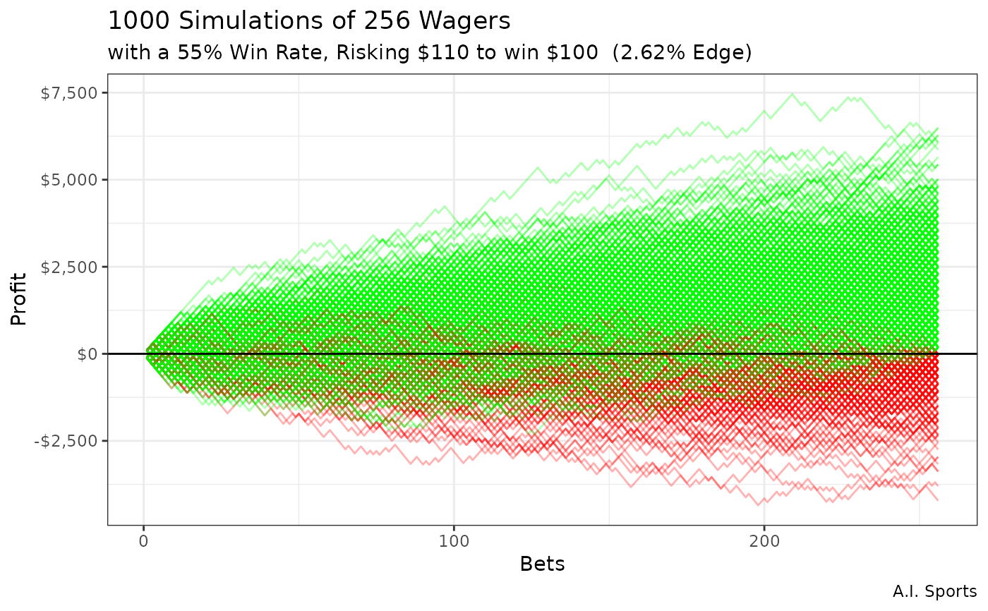
bankroll_plot(
bets = 256,
win_rate = 0.55,
bet_size = 100,
sim_length = 1000,
avg_odds = -110,
odds_type = "us"
)
#>
#> Positive Negative
#> 0.776 0.224
#>
#> Median Profit/Loss = $1,450
#> Warning: The `guide` argument in `scale_*()` cannot be `FALSE`. This was deprecated in
#> ggplot2 3.3.4.
#> ℹ Please use "none" instead.
#> ℹ The deprecated feature was likely used in the bettoR package.
#> Please report the issue at <https://github.com/papagorgio23/bettoR/issues>.
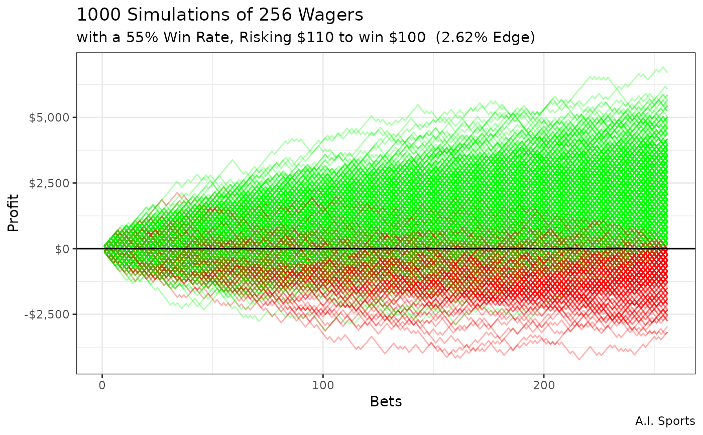 bankroll_plot(
sim_length = 500,
avg_odds = -110,
win_rate = 0.5455
)
#>
#> Positive Negative
#> 0.746 0.254
#>
#> Median Profit/Loss = $1,240
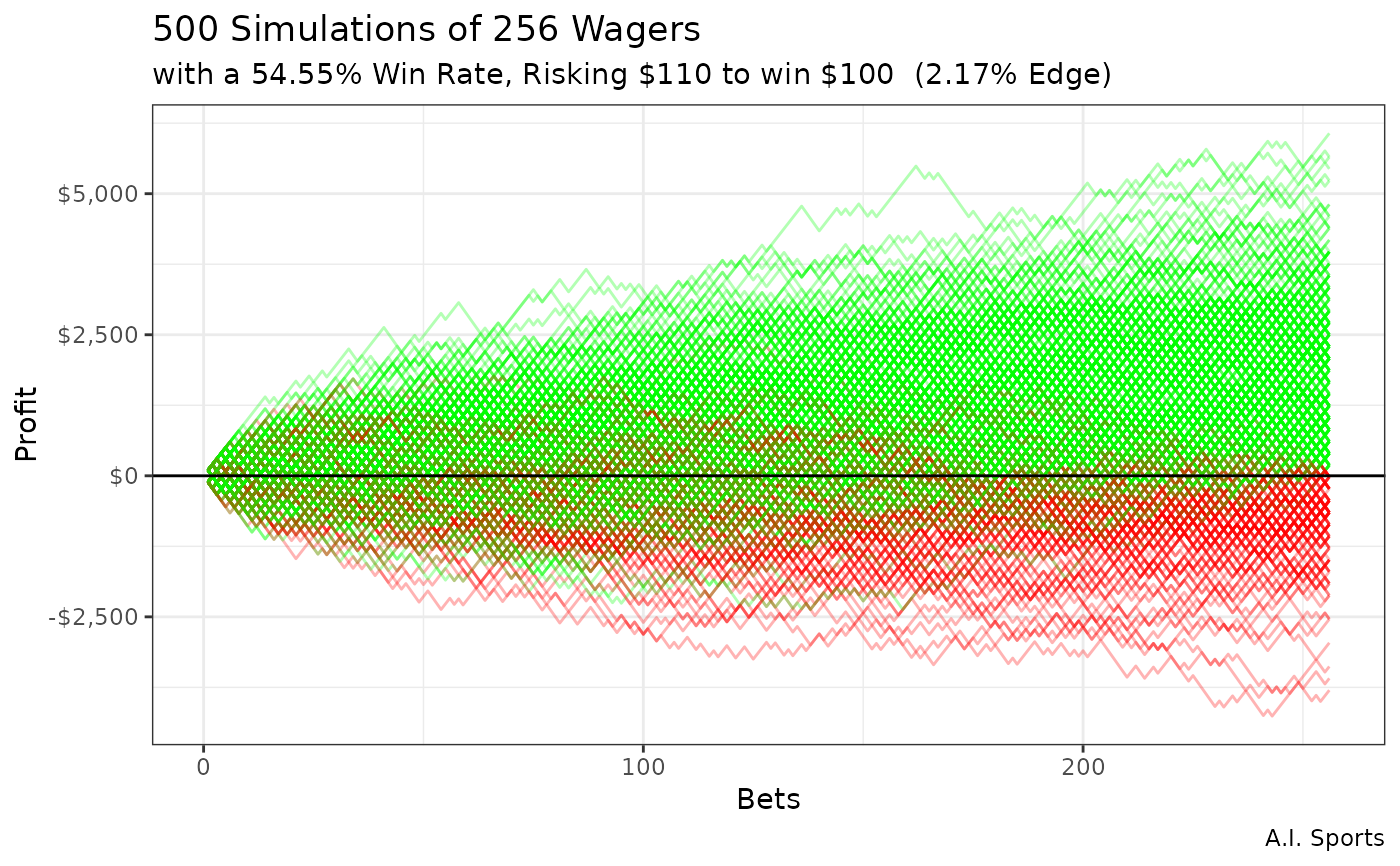
bankroll_plot(
sim_length = 500,
avg_odds = -110,
win_rate = 0.5455
)
#>
#> Positive Negative
#> 0.746 0.254
#>
#> Median Profit/Loss = $1,240
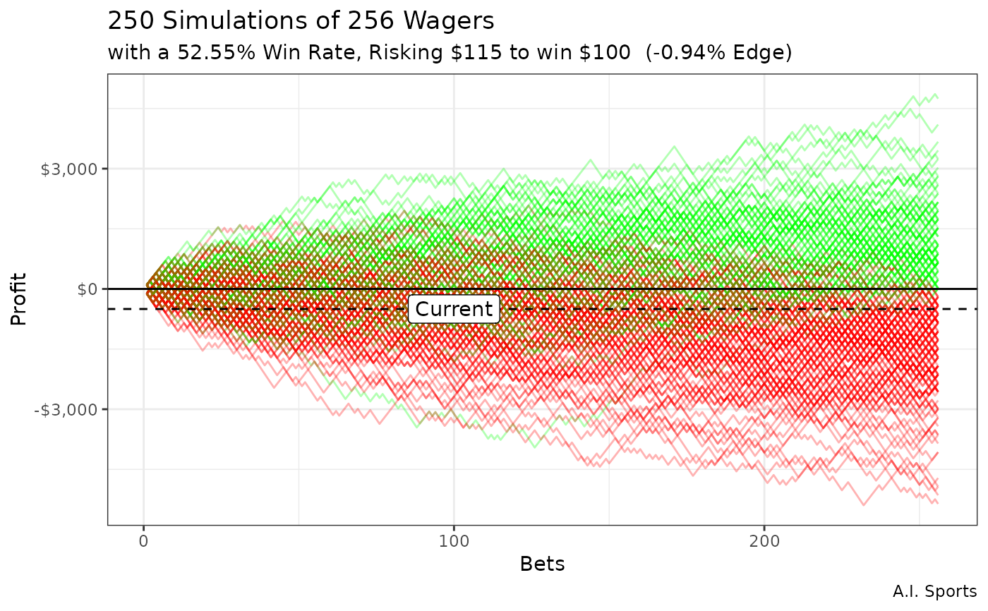
 bankroll_plot(
sim_length = 250,
avg_odds = -115,
win_rate = 0.5255,
current_bet = 100,
current_win = -500
)
#>
#> Positive Negative
#> 0.4 0.6
#>
#> Median Profit/Loss = -$630
bankroll_plot(
sim_length = 250,
avg_odds = -115,
win_rate = 0.5255,
current_bet = 100,
current_win = -500
)
#>
#> Positive Negative
#> 0.4 0.6
#>
#> Median Profit/Loss = -$630
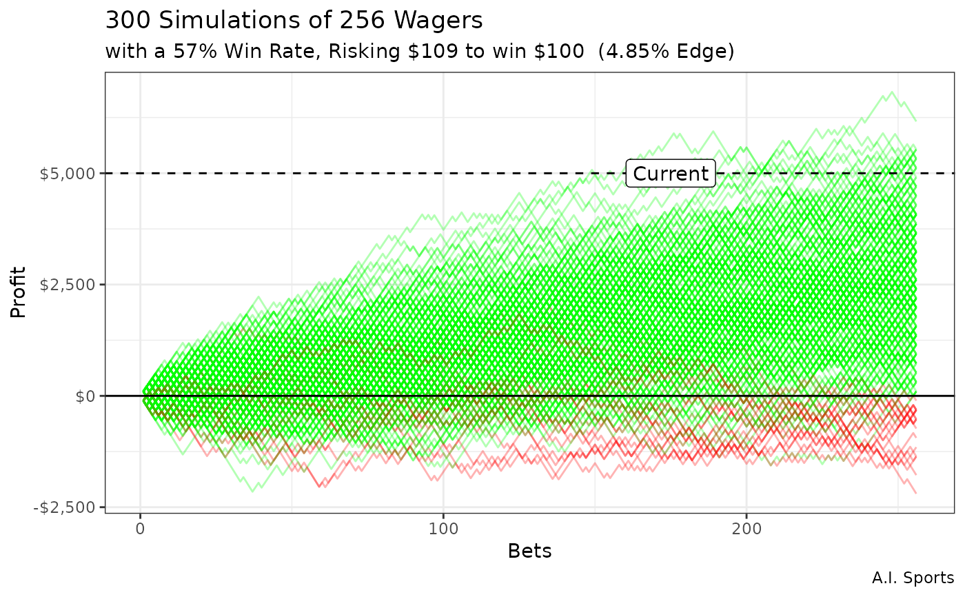
 bankroll_plot(
sim_length = 300,
avg_odds = -109,
win_rate = 0.57,
current_bet = 175,
current_win = 5000
)
#>
#> Positive Negative
#> 0.93 0.07
#>
#> Median Profit/Loss = $2,401
bankroll_plot(
sim_length = 300,
avg_odds = -109,
win_rate = 0.57,
current_bet = 175,
current_win = 5000
)
#>
#> Positive Negative
#> 0.93 0.07
#>
#> Median Profit/Loss = $2,401
 bankroll_plot()
#>
#> Positive Negative
#> 0.796 0.204
#>
#> Median Profit/Loss = $1,450
bankroll_plot()
#>
#> Positive Negative
#> 0.796 0.204
#>
#> Median Profit/Loss = $1,450